Earned Value Management (EVM) in Agile Development

In this article, we are going to explore Earned Value Management (EVM), a widely used traditional management technique, but we are going to look at it within the context of an Agile domain.

Let’s consider an example scenario. A product manager, who works for a large aircraft manufacturing organization in the United States, follows a hybrid model of development and, with his team, releases a new version of aircraft handling software every couple of weeks. At the start of each iteration, he may be unsure about the applicability of earned value analysis, measurement, and management within Agile. His main questions may be:

• How can we apply EVM while following an Agile approach? Is it natural?
• With frequent scope changes, how does one determine what to measure against?
• Scope change is also frequent on the iteration level! How can we incorporate EVM metrics in such cases?

To understand EVM, one needs to understand the concept of baseline, first and foremost. In EVM terminology, baseline is further defined as the performance measurement baseline (PMB). Let’s first define PMB, because, as I’ve seen, the lack of clarity regarding EVM is typically due to lack of PMB understanding. 

Performance Measurement Baseline (PMB)

The PMB is a virtual (not physical) baseline integrating scope, schedule, and cost baselines. In other words, PMB is the time-phased budget of authorized work for a project or program.

EVM is fundamentally based on this baseline–irrespective of chosen life cycle, be it predictive (Traditional), adaptive (Agile), or any other. It doesn’t matter how many iterations (or sprints, if in Scrum) you have or how frequently the scope changes. For EVM, it matters where and how you are setting your baseline. We will see shortly where the baseline is an Agile context. As EVM integrates scope, schedule, and cost, it’s quite a powerful technique. This is shown in the below figure.

 

Another issue occurs when management practitioners incorrectly interpret earned value as being business value. Earned value is not business value, rather it’s the value that you have earned in terms of money after completing the work. Hence, it’s actually a measure of work performance or performance against the set baseline or PMB.

With these fundamentals in mind, let’s now consider the foundational metrics in EVM. 

Foundational Metrics in EVM

The foundational metrics in traditional EVM are noted in the below table. I call them the foundational (or basic) metrics, because, based on these metrics, current and future performance metrics are derived.

As you go through the metrics in EVM, one key thing is to remember is this: everything is in terms of money. The budget, of course, will be in terms of money, and the work planned and work performed or executed, will also be in terms of money in this case.

We will look at the usage of these foundational metrics for Agile development shortly. Note that with these foundational metrics in place, we derive performance metrics of EVM.  

Current Performance Metrics in EVM

The current performance metrics used to calculate EVM are noted in the below table for a Traditional environment. I call these metrics current performance metrics, because the measurement happens on the status date, data date, or record date. The good news is, that these foundational metrics remain the same for Agile projects and/or programs.  Keep reading, as we are going to reuse these performance metrics in the next section.

It’s pertinent to note the behavior of SV and CV. If they are positive or negative, then the project or program is ahead of or behind schedule and cost, respectively. Similarly, if SPI and CPI are above or below 1.0, then the project or program is ahead of or behind schedule and cost, respectively. 

Using EVM in Agile Approaches

When using EVM in an Agile approach or environment, we circle back to the concept of baseline. In Agile projects, the baseline at the release level, not at an iteration level must be considered.

You may be wondering why. In Agile approaches, work is considered “done” at the end of each iteration (or sprint). While it’s true that story points are used to relatively estimate work items being taken-up, work is not considered to be fully “done” until the end of the iteration. If an item is not done, then it’s usually pushed into the next iteration. Hence, measurement during an iteration adds no value. This is because the work can’t be complete/done (or incomplete/not-done) mid- iteration.

If a story is complete, only then is it considered “done.” If a story is partially complete, (say only transition testing is remaining, then it’s not considered to be “done” at all). As you can see, it’s futile to have a baseline at an iteration level.

Are you wondering now how to calculate the performance measurement baseline (PMB) at a release level?

Simply add up the number of story points that you have planned for the release. While the PMB is at the level of the release, we do the measurement at the end of every iteration. In other words, our status date or data date is set for the end of the iteration. This is because, at the end of the iteration, we know the amount of work completed or “done.” And, this work counts towards velocity. Velocity, as explained in this article, also can inform the number of iterations in a release. You can decide to have measurement at the end of any iteration – iteration 1, iteration 2, and/or iteration-N.

A (product) backlog-based representation with earned value related calculations is depicted in the figure below.

As shown, the EV, PV, and AC values are calculated on the status/data date, which occurs at the completion of the iteration. The PMB is set for the release, and this also informs the budget at completion (BAC) for the release.

Next, we will consider the metrics associated with EVM in an Agile environment. 

EVM Metrics in Agile Approaches

The foundational EVM metrics used in Agile are noted in the below table with explanations. As you can see, the traditional metrics of EV, PV, AC, and BAC are also taken-up in Agile development; however, the explanation and understanding with respect to Agile contexts are different.

The values for PV, EV, and AC are calculated at the end of every iteration (you can set the status date as of the end of the concerned or considered iteration), whereas the BAC is determined at the release level. This is in sync with the backlog-based representation that we saw earlier.

The budget at completion (BAC) at the release level will be calculated as follows:

Budget at Completion (BAC)

= Total budget for the release

= Number of Items in the Release * Cost per backlog items (or cost per PBI)

For every item in the backlog (PBIs), cost is usually considered, which is one of the key product prioritization factors.

Now that we have the BAC, we can easily calculate the EV and PV, respectively with the below formulas:

First taking PV, the formula will be:

Planned Value (PV)

= Percentage of planned complete * BAC

= % of planned complete * BAC.

Earlier I said, PV, EV, and AC, etc. are calculated as of the status/data date or the iteration completion date. Considering an scenario where you have five iterations in a release and you are measuring at the end of the 2nd iteration, we’d see the following: case:

Percentage (%) of planned complete

= Iteration number / Number of iterations

= 2/5

= 40%

The formula for earned value (EV) will come out as shown below.

Earned Value (EV)

= Percentage of actual complete * BAC

= % of actual complete * BAC.

Why are we considering percentage of percentage of actual complete for EV? It’s because earned value is the value that you have earned by completing the work or having “done” the work.

To determine the percentage of actual completed work, you have to consider the stories that have been completed at the end of an iteration. Let’s say you have completed 40 story points worth of work out of 200 in a release, and you’re at the end of 2nd iteration. The percentage is calculated as follows:

Percentage (%) of actual complete

= Story points completed (or done) / Total story points

= 40/200

= 20%

I’ve summarized the calculations in the below table. 

So far, we have shown small examples with respect to BAC, PV, EV, and AC. Based on these metrics, we can easily calculate the current performance metrics of SV, CV, SPI, and CPI using the formulas mentioned in Table – 2.

For this purpose, let’s take an example from the course, ACP Live Lessons, Guaranteed Pass, to compute the associated metrics. A dedicated set of videos are available in the Live Lessons course.

An Example – EVM In Agile

A project is being released in an Agile mode. Below are the details for the project:

• Product Backlog = 500 story points
• In the first release = 200 story points
• Velocity = 25 points per iteration
• Cost per point = $1600
• At the end of 1st iteration, actual cost incurred was $30,000.
• At the end of 1st iteration, story points completed were 20 story points.

With this, we can determine the following.

• Budget at Completion (BAC)
• Number of Iterations
• Planned value per iteration (PV) and Earned Value (EV) for the first iteration
• Schedule Variance (SV) and Cost Variance (CV)
• Schedule Performance Index (SPI) and Cost Performance Index (CPI)

If you have understood so far, you can try it on your own and determine the values being asked in the above questions.

To confirm your understanding and reaffirm your answer, the solution is noted below.

Budget at Completion (BAC)

= Cost per point * Number of story points

= $1600 * 200

= $320,000

Total number of Iterations

= Story points in a release / Velocity

= 200 / 25

= 8

Percentage (%) of planned complete at the end of first iteration

= Iteration number / Total number of iterations 

= 1 / 8

= 12.5%

Percentage (%) of actual complete at the end of first iteration

= Total number of story points completed / Total number story points planned

= 20 / 200

= 10%

Now that we have the needed values, let’s calculate the other associated metrics of PV, EV, and AC.

Planned Value (PV) for the iteration

= % of planned complete * BAC

= 12.5% * $320,000

= $40,000

Earned Value (EV) for the iteration

= % of actual complete * BAC  

= 10% * $320,000

= $32,000

The actual cost (AC), as mentioned in the question

= $30,000.

With these calculations, we can now determine the current performance metrics of the project at the end of the first iteration.

Schedule Variance (SV)

= EV – PV

= $32,000 – $40,000

= – $8,000

Cost Variance (CV)

= EV – AC

= $32,000 – $30,000

= + $2,000

Look at Table – 2. One could say the release is behind schedule and under budget by looking at the performance metrics of SV and CV, respectively. This is because SV is negative (bad), whereas CV is positive (good).

Next, let’s determine the values for SPI and CPI.

Schedule Performance Index (SPI)

= EV / PV

= $32,000 / $40,000

= 0.8 

Cost Performance Index (CPI)

= EV / AC

= $32,000 / $30,000

= 1.07

Again, referring to Table – 2, you could say the release is behind schedule and under budget by looking at the performance metrics of SPI and CPI, respectively. This is because SPI is below one (bad), whereas CPI is above one (good). 

Representation in S-Curve

Like a traditional EVM, in Agile context, you can also depict the various EVM metrics in an S-curve. These curves are frequently used in many projects to depict the progress and status reporting. However, your perspective has to change/adapt for the Agile context.

An S-curve showing BAC, EV, PV, AC, SV, and CV is shown in the below figure. 

The BAC is at the release level. The PMB line is along the EV curve. Our status date or data date is at the completion of Iteration – 3, and, on this date, we are measuring the foundational metrics of PV, EV and AC, as well as the current performance metrics of SV, SV, and hence, associated SPI and CPI. When you combine this representation with estimated story points in the product backlog, you can have the release burn-up chart. 

Video – EVM in Agile

As we close, I want to summarize the foundations of EVM in Agile in the below video, taken from the course, ACP Live Lessons [duration: 13m:06s]. This video notes certain key points you should keep in mind when calculating earned value in an Agile domain. It also further explains the above S-curve. For the best experience, you may want to go full-screen in HD mode and plug-in your earphones.

With this, I believe, I leave you with the fundamentals of earned value management executed in Agile environments.

If you have comments, suggestions, or new ideas, please do share them below.

--

This article was first published by MPUG.com on 22nd September, 2020. This is a refined version.

References

[1] Course: ACP Live Lessons, Guaranteed Pass or Your Money Back, by Satya Narayan Dash

[2] Book: I Want To Be A PMI-ACP: The Plain and Simple Way, 2nd Edition, by Satya Narayan Dash

[3] Course: ACP 21 Contact Hours, with Money Back Guarantee, by Satya Narayan Dash

Risk Attitude and Risk Attitude Spectrum

Risk attitude, risk appetite, risk tolerance, and risk threshold are all separate and distinct terms. Understanding of these terms are foundational in risk management and to conduct proper risk management in the real-world. 

In this article, we will see these terms with examples, figures, explanations and video. The content for this article is taken from my new course, RMP Live Lessons, Guaranteed Pass. 

Attitude, put simply, is the thinking and approach, which are displayed in behaviors. Attitude is obviously displayed by people or persons involved in any work. Considering projects, attitude will come from the stakeholders of the project.

A project is almost always executed in an uncertain environment. Uncertainties lead to risks, which can positively or negatively impact the project objectives. Hence, we have to address those risks.

Now, attitude is displayed by stakeholders for many aspects of project such as quality (e.g., high quality or high grade), processes to be undertaken (e.g., heavy set of process or "just-enough" processes), life cycle to be selected (e.g. waterfall, agile or hybrid). Similarly, stakeholders will also have attitude towards project risks. Some stakeholders may not like risks at all, while few others may be very comfortable with a large number of risks.

Risk Attitude determines the extent to which individual risks or overall project risk matters. The Foundational Standard for Risk Management in Portfolios, Programs and Projects from the Project Management Institute (PMI®) defines Risk Attitude as follows:

A disposition toward uncertainty, adopted explicitly or implicitly by individuals and groups, driven by perception, and evidenced by observable behavior.

In other words, you can say a risk attitude basically informs how stakeholders behave towards the uncertainties. The risk attitudes of the stakeholders may be influenced by a number of factors such as:

• Organizational Culture
• Scale of Project
• Strength of Public Commitment
• Environmental Impact 
• Industrial Relations

Stakeholders in a project will have different risk attitudes and also a stakeholder’s risk attitude varies throughout the project life cycle. Hence, their needs and expectations on risks should be properly managed. But why would you need that?

Because perception forms the attitude. Attitude results in behavior. And behavior will have consequences. 

As shown above, perception drive attitude, which in turn drives behavior resulting in consequences. 

Risk Attitude: Risk Averse and Risk Seeker

The risk attitude of stakeholders can range from risk averse to risk seeker. 

Risk Averse: Stakeholders with very low risk appetite and these stakeholders feel very uncomfortable in the presence of uncertainty. 

Risk Seeker: Stakeholders with high risk appetite and these stakeholders view uncertainty as a welcome challenge. 

Risk attitude is expressed in 3 themes:

• Risk Appetite: It is the degree of uncertainty a stakeholder is willing to take in expectation of a reward.
• Risk Tolerance: It is the degree of uncertainty a stakeholder will withstand (typically expressed in range). This is not as frequently used as risk appetite and risk threshold in the latest trends of risk management. It’s deprecated. 
• Risk Threshold: It is the highest level of risk tolerance. Below the threshold, risk will be accepted. Above the threshold, risk won’t be accepted by stakeholders.

Risk threshold is the measure of acceptable variation around an objective that reflects the risk appetite of the organization and stakeholders. 

Examples: Risk Appetite, Risk Tolerance and Risk Threshold

Let’s take some examples to understand. 

Risk appetite and threshold values are set during risk management planning. This is pre-decided by managers above the project manager. However, these can be customized/set for an individual project with stakeholder analysis.

Risk appetite and threshold values for the individual project risks are calculated as numbers, e.g., 9, 11 or 15, during qualitative analysis. It also can be scaled textuals such as low, high, very high etc.

Risk tolerance is typically expressed in range, e.g., we will accept up-to 10% variation in cost, or we can accept up-to 30-days-delay in the project schedule.

The risk threshold reflects the risk appetite, as we saw earlier. Hence, a risk threshold of +/-10% around a cost objective reflects a higher risk appetite than a risk threshold of +/-5%. Similarly, one can consider other objectives.

There can be other examples of Risk thresholds, some of which are noted below.

• Consider a risk’s exposure (potential impact). If the potential impact is below a minimum level, then it won’t be included in the Risk Register. In other words, the risk threshold value, related to minimal risk exposure, is not crossed.
• Qualitative or quantitative definition of risk rating or risk score. The risk score is the multiplication of risk probability and impact. Considering qualitative risk definition, if the risk score is less than 9, then the risk threshold value is not crossed.

You can understand with more examples, you can refer to this PMP Protein Article.

Risk Attitude Spectrum

It is evident that stakeholders of a project will be different - not everyone thinks alike. Hence, the risk attitude will also be different. After all, risk attitude informs how a stakeholder perceives a risky situation – favorably or unfavorably. So, risk attitude may not be stable, or homogenous across the stakeholders. Risk attitudes, as we just came to know, are not homogenous among the stakeholders. It may also change over the life cycle of the project or program or portfolio. 

The same uncertain situation can result in different kinds of behavior from stakeholders depending on how they perceive the uncertainty. An uncertain situation, which is considered to be too risky for one stakeholder, may be accepted easily by another stakeholder. 

Consider the above aspects of stakeholders, many risk management practitioners conclude that risk attitudes actually exist on a spectrum – from very low or low risk-taking ability to high or extreme risk-taking ability. The spectrum of risk attitude for the stakeholders is shown in the below figure. 

As shown in the above figure, the responses to uncertainty and comfort/discomfort level of stakeholders are shown in X and Y axes, respectively. The risk tolerant ones have little/low or no comfort/discomfort level when uncertainty happens or arises. 

Video: Risk Attitude Spectrum

Let's have a relook at the previous graph. With an increase of comfort level reaching “high”, the stakeholder can be considered to be risk seeking or risk seeker. On the other hand, when the discomfort level is high, then the stakeholder can be considered to risk averse. Similarly, when there is an extreme level of comfort with uncertainty, the stakeholder will be termed as risk addicted. On the other hand, with an extreme level of discomfort, the stakeholder will be termed as risk paranoid.  

This is further explained in the below video [duration: 2m:44s], taken from RMP Live Lessons, Guaranteed Pass. You may want to plug-in your earphones to have a better experience. 

Conclusion

While preparing for the RMP Exam, you have to very familiar and conceptually clear about the below terms:

• Risk Attitude
• Risk Appetite
• Risk Threshold
• Risk Exposure
• Risk Rating
• Risk Value
  
• Risk Score, among others.

Some the above terms are actually quite the same, but can differ based on the contextual application! 

Coming to the Risk Management Professional (RMP®) exam, questions are rarely direct. They will be mostly situational. With a strong foundational understanding and sufficient practice, you can easily answer them. 

References:

[1] Course: RMP Live Lessons, Guaranteed Pass or Your Money Back, by Satya Narayan Dash, CIPSA, CHAMP

[2] Book: I Want To Be A RMP: The Plain and Simple Way To Be A RMP, 2nd Edition, by Satya Narayan Dash, CIPSA, CHAMP

[3] Course: RMP 30 Contact Hours with Money Back Guarantee, by Satya Narayan Dash, CIPSA, CHAMP

End to End Risk Management with MS Project and Primavera Risk Analysis

Imagine you are managing a large project, which is strategically important and complex. At the outset, you realize there will be a number of risks, which if not managed well, could paralyze the outcome and have negative impacts on the project objectives. You want to proactively identify, analyze, respond, track, and monitor your project’s risks. And, it would be great to have a dedicated risk management tool to use alongside your project management software.

What are your options? Will software tools like Excel help? Will a software tool for only project management meet your needs?

If you have ever managed risks, you know a spreadsheet is not the answer. A spreadsheet is not at all designed for project management–let alone risk management. It’s likely that a project management software tool only meets your need half-way.

One of the most frustrating experiences faced by management practitioners with respect to software tools and one response was related to risk management and tracking, specifically in a scenario where spreadsheets were being used. Another aspect that came to light was the need for an integrated and risk-adjusted schedule-cost management system, which brings up questions like: what are the duration estimates and cost estimates associated with the risks? How can a PM manage risks in with a single, centralized tool?

In this piece, I’d like to present an integrated approach to project management with strong end-to-end risk management capabilities. For this purpose, I’ll be using two software tools:

• Microsoft Project (MSP) 2019 for project management, and
• Primavera Risk Analysis (PRA) 8.7.5 for risk management.

The practical examples and samples for this article have been taken from Practical RMP with Primavera Risk Analysis, whereas the theoretical explanations are from RMP Live Lessons.

Let’s start with creating a project plan with MS Project. 

Create the Project Plan

While you can directly use PRA to create your project plan, most project managers use MSP frequently for planning because of its simplicity, ease of use, and user friendliness.  For this reason, we will create the plan first in MS Project. The plan depicted in the below figure.

The statistics of the project are these:

• Duration: 38 days
• Cost: $67,680 USD
• Finish Date: June 30, 2021 (06/30/21)

The project is the creation of a Smart Site and involves multiple resources.

Do note that if you have modified the calendars for the project and/or have added custom calendars, you’ll need to ensure you have the corresponding calendars in PRA.

Set-up PRA for Risk Management

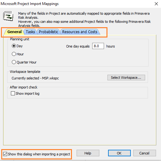
Before importing the plan, ensure that the settings for MS Project in PRA are correct. This can be opened by going to PRA tool’s File à Microsoft Project à Edit Default Import Mapping… menu.

Keep the “Show this dialog…” checkbox enabled so that when you open the MSP Plan in PRA, you can have a quick look at the settings before actual import happens.

Import the MSP Plan into PRA

Now that we have set the MSP related settings in PRA, we will import the project plan created in MSP into PRA. It will happen in a few seconds. Post import, in PRA, the plan will be shown as below.

The imported project plan in PRA has the following statistics:

• Remaining Duration: 38 days
• Remaining Cost: $67,680 USD
• Finish Date: June 30, 2021 (06/30/21)

This is perfectly in sync with the statistics of our project plan created earlier in MSP. It’s also a good idea to check a few of the tasks in the project to see that the import has happened properly. In our case, the task/activity “PRD Preparation” has been considered. It matches perfectly with the MSP Plan considering Dates, Resources, and Cost, among other fields.

Important Notes

At this stage, I’ll recommend that you read this Risk Management Framework for Projects article to understand how risks are managed and monitored over various Risk Management processes. Here, I’ll be using only the Risk Register, not the Risk Report.

In addition, I’ll explain some key points with respect to risk management, which will help you to understand why I’ve taken the following steps and performed the associated activities. Take a look at the video [Duration: 4m:12s] below—it’s been taken from RMP Live Lessons. For a better experience, you may want to go full-screen with HD mode and plug-in your earphones.

Risk Identification and Risk Register

Now, we are going to prepare the Risk Register. Preparation of this key project artifact happens during the Risk Identification process.

To create the Risk Register with PRA software, go to Risk à Register… menu, or click on the Risk Register icon on the Risk Toolbar of PRA. The Risk Register creation dialog box will pop up, and we will use the standard risk register option.

 

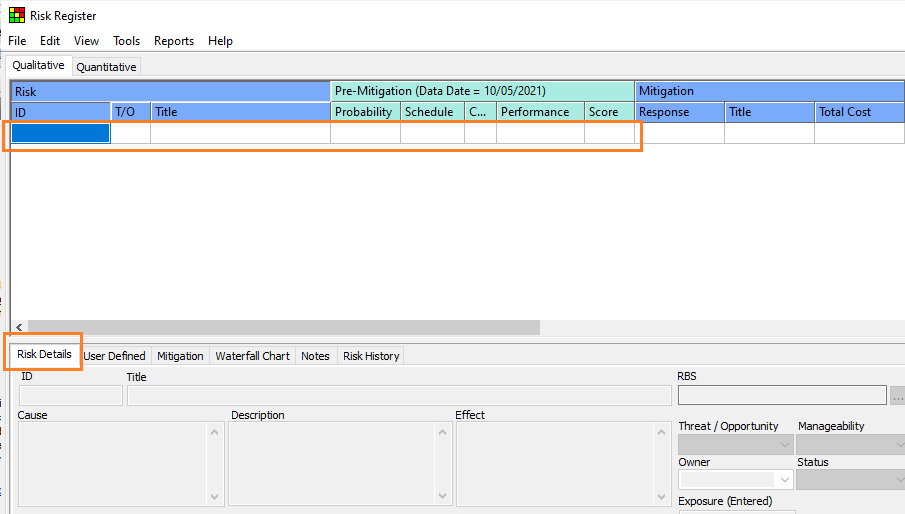
When the standard Risk Register first opens, of course, it will be empty as shown below.

You can enter new risks easily by adding details for the identified individual project risks.

As you can enter the risks, provide all the needed information such as Risk ID, Threat or Opportunity, Risk Title, the Pre-mitigation information such as Probability scales, Impact Scales, etc. You can also add the Risk Details such as Cause, Effect, and Risk Category, among others.

As shown, we have four identified risks (threats) for this project with their respective details entered. The cause, effect, description, owner, RBS type, and status values have been entered for each of the risks.

Do not worry about the risk responses now. We will address them in the step for risk response planning as I explained in the earlier video. The risk score is calculated by taking the risk parameter values from the Risk Probability and Impact (PI) Matrix. For the sake of this example, I’ve used the following matrix.

The probability and impact scales notations in the Risk Register are these:

• Very Low (VL)
• Low (L)
• Medium (M)
• High (H)
• Very High (VH)

As you multiply the probability and impact values, you will get the Risk Score. For more depth, refer to this detailed article on Risk Matrix Reporting.

Risk Qualification

Our next step is to qualify these individual risks. We will determine the probability and impact values of these risks. You can have other risk assessment parameters, as well, such as Risk Manageability or Risk Proximity, among many others.

Considering the probability and impact values of these risks, as we qualify them, the Risk Register will be updated as shown below.

As you can see, the current Risk Register has seen a number of updates. Considering Risk ID – 001, some of the key updates are:

• Risk Score is now 21. (change from 72 to 21)
• Risk Owner is confirmed. (John R is the confirmed owner)
• Risk Status has been modified. (Status is “open” now; earlier “proposed”)

Similarly, we have also qualified other individual project risks: Risk 002, Risk 003, and Risk 004.

Risk Quantification

This step of risk quantification is optional, as we have seen in the RMP video. Though our project is a simple one, let’s do risk quantification for one individual risk (Risk 001: Poor understanding of design specification). After quantification of this risk, the pre-mitigated Quantified Risk Register will show as follows:

Note that Risk 001 has now been quantified from a schedule perspective by associating it with two tasks in the Project Plan, i.e. Task ID 000009 and Task ID 000010, from “Phase – 1” under the WBS element of “Design and Development Phase” at Level – 2 of the work breakdown structure (WBS).

I’ve used BetaPert probability distribution for the tasks mentioned and have entered the minimum, mostly likely, and maximum duration estimates. Similarly, you can also quantify with respect to cost estimates.

Post quantification, you can do a variety of analyzing such as:

• Monte Carlo Analysis,
• Criticality Analysis,
• Probabilistic Branching and Analysis, and
• Sensitivity Analysis, among many others.

Risk Response Planning and Response Integration

Next, we will do the risk response planning for the individual risks to bring down the probability and/or impact values of these risks. With this, we can keep the risk score within the risk threshold.

For this purpose, we again have to go to the Risk Register and modify the risk response strategies along with the associated risk response actions. The modified risk register is shown below.

 

Considering “Risk 004: Key resources unavailable,” the Risk Score has been reduced from 56 to 1, and similarly for certain other risks.

For Risk 004, the associated actions are noted under the highlighted “Mitigation” tab. There are two mitigation response actions:

• Risk Response Action – 1: Get the resources from other functional departments.
• Risk Response Action – 2: Prioritize project resources.

The assigned risk response owners and associated cost are noted. The associated cost also reflects on the top panel for Risk 004.

Risk Monitoring and Tracking

Our final step relates to risk monitoring and tracking. During risk monitoring, new risks may be identified, an existing risk status can change, an existing risk can become obsolete, or an existing risk may not occur.

Let’s say a new positive risk (opportunity) is identified, and we need to add this risk into the register. As we have seen earlier, risk management is both iterative and integrative in nature. 

As shown, we now have a new risk—“Risk 008: Reuse of previous design module.” As this risk is freshly detected, default values have been populated. The blue letter “O” represents an opportunity.

Subsequently, we have to determine the initial characteristics of this risk, followed by qualification and quantification (optional), and have the needed risk response strategies with associated risk response actions. Finally, we have to monitor this new adjusted risk with response and associated actions.

As we reach the end of this article, some of you may be thinking can this risk register be exported to MS Excel? After all, not all stakeholders will have MS Project 2019 and Primavera Risk Analysis software installed.

The answer is yes! You can export the Risk Register to MS Excel by going to Risk Register’s File à Export Risk Register As… menu. From there, while saving, choose “Microsoft Office Excel (.xls)” option to save.

With this process in mind, I believe you will have a sound understanding of end-to-end risk identification, analysis, response planning, and implementation, followed with risk monitoring and tracking.

 

--

This article was first published by MPUG.com on 18th May, 2021.

References:

[1] Online Course: Practical RMP with Primavera Risk Analysis, by Satya Narayan Dash

[2] Online Course: RMP Live Lessons, Guaranteed Pass, by Satya Narayan Dash

[3] Online Course: MS Project Live Lessons, by Satya Narayan Dash